
There are a lot of well-established run estimators out there that are quite accurate for estimating the overall run production of major league baseball teams of the last few decades. None of these have an explicit dependence on OBP (On-base percentage) like EBP does. However, as I mentioned in What the OBP-dependence of established run estimators probably looks like, when I realized that most or all of them should have an implicit dependence on OBP that should also exhibit the Fixed Outs Explosion, I set out to see just what that dependence looked like. I would have to create estimates of how each of the inputs used by these formulas (AB, hits, walks, strikeouts, etc.) vary with p (the probability of a hitter reaching base in any plate appearance, approximated by OBP). In this article I detail how I went about doing that.
Please note that this is just one way to go about it. These estimations could certainly be improved upon, with enough effort and analysis of data. For example, the fraction of base reaches that are home runs should probably not be constant with p; it should probably be higher for low values of p. This is because home runs (and manufactured runs) are pretty much the only ways to score runs at very low values of p, so hitters will bias their approaches toward hitting home runs in lower-p environments. But I didn’t do that. I assumed that the home run fraction would be constant across all p, in part because I can’t make a strong case that any other estimation would be more accurate, and in part because the extra complication this would bring did not seem worth the effort just now.
Overview of approach
Originally I figured that:
- base reaches would vary like OBP times plate appearances;
- outs would vary like (1 – OBP) times plate appearances;
- and plays that require runners on base before they happen (grounding into a double play, stealing a base, etc.) would vary like OBP(1-OBP) times plate appearances.
Of these, the third assumption didn’t turn out well. I would have to replace the first factor, OBP, with a better factor for representing how likely it is that there is a runner on base when a batter comes to the plate. I ended up using PRO(p) = 1.95p/(1+1.1p) for this factor (PRO as a acronym for the Probability of a Runner On). So these plays then varied like

or just

But the key to everything was getting plate appearances right, or at least very good. That’s because plate appearances PA(p) is a component of the calculation of every other input I mocked for the run estimator formulas. Even more critically, it’s the component that provides the Fixed Outs Explosion to every other statistical input. Run production explodes when p gets near 1 because all the base-reach stats (hits, walks, etc.) explode when p gets near 1, and these explode because plate appearances does. It all hinges on this one amount – PA(p) drives the Fixed Outs Explosion.
Definitions
I should state clearly what I mean by PA(p), and some other expressions I’m about to use. So here are some definitions:
PA(p) is the number of plate appearances you expect to have for a particular value of p between 0 and 1, for the team in question.
PA0 is the number of plate appearances that actually occurred during the season for the team in question.
We will follow this same naming pattern for all other quantities named here.
PA(p) and PA0 are numbers of plate appearances.
OOB(p) and OOB0 are numbers of outs made on the bases.
OAP(p) and OAP0 are numbers of outs made at the plate.
FO(p) and FO0 are the fractions of those reaching base who make outs on the basepaths.
OutsMade: overall number of outs made is considered to be a constant that does not vary as p changes. We therefore simply refer to it as OutsMade.
Deriving the dependence of plate appearances on p (PA(p))
Overview: the two parts
We will now derive an expression for plate appearances as a function of p (that is, PA(p)) in terms of p and team statistics that we can look up. We’ll begin with the relationship
OutsMade = OAP(p) + OOB(p),
which should need no explanation. (Note that this adds in a bit of realism not contained in the EBP formulas, which presume no outs on the bases. Effectively, for EBP, we’re using simply
OutsMade = OAP(p)
instead.)
We’ll proceed by substituting in expressions for OAP(p) and OOB(p) that include PA(p) in them, then solving for PA(p).
Finding the first part
OAP(p) is easy: we just use OAP(p) = (1-p)PA(p).
Finding the second part, step 1: fraction of baserunners making outs
To get OOB(p), we’ll multiply the number of base reaches by the fraction of those who reach base who make an out on the basepaths. The first part of this product, base reaches, we have already assumed to equal p(PA(p)), so we have that part done. The other part of the product is FO(p), the fraction of baserunners who make an out; we need to make our best guess at a curve for that.
We assume FO(p) goes down as p goes up, because baserunners will become less daring when p is high, due to the higher costs of an out relative to each base advance. But we also assume it does not go down dramatically. I plotted data points FO0 = OOB0/BR0 versus p0 for actual teams of the last 60 or so years, looking for a trend that hints at what FO(p) should look like. Exponential curves seemed to give more sensible results than linear ones. A curve through the middle worked out to

The exponent is almost exactly 2, so I just made it 2, as that’s easily correct within the accuracy of our dataset. The .227 “scaling factor” can be adjusted team-by-team. Multiplying the above equation by 

Drop the .227 to allow for this value varying team to team:
Because the scaling factor is a constant for a particular team, it’s the same for all values of p, so we can use any value of p to calculate it. By using p0, we’ll have everything in terms of quantities we can look up.
Scaling Factor for particular team =

As we saw just above, the general FO(p) is just this times 

Finding the second part, step 2: reassembling
Now that we have FO(p), we can use it to construct OOB(0):

Dividing by OOB0 puts this in a form I’ll use frequently, which shows a proportionality relationship:
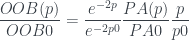
Summing both parts and solving for PA(p)
But right now we need the OOB(p) form. With that, we go back to the equation we started with, and can finally substitute in what we’ve come up with and get to a formula for PA(p):
![OutsMade = OAP(p)+OOB(p) = (1-p)PA(p) + OOB0 \dfrac{e^{-2p}}{e^{-2p0}} \dfrac{PA(p)}{PA0} \dfrac{p}{p0} = [ (1-p) + \dfrac{OOB0}{PA0} \dfrac{e^{-2p}}{e^{-2p0}} \dfrac{p}{p0} ] * PA(p)](https://s0.wp.com/latex.php?latex=OutsMade+%3D+OAP%28p%29%2BOOB%28p%29+%3D+%281-p%29PA%28p%29+%2B+OOB0+%5Cdfrac%7Be%5E%7B-2p%7D%7D%7Be%5E%7B-2p0%7D%7D+%5Cdfrac%7BPA%28p%29%7D%7BPA0%7D+%5Cdfrac%7Bp%7D%7Bp0%7D+%3D+%5B+%281-p%29+%2B+%5Cdfrac%7BOOB0%7D%7BPA0%7D+%5Cdfrac%7Be%5E%7B-2p%7D%7D%7Be%5E%7B-2p0%7D%7D+%5Cdfrac%7Bp%7D%7Bp0%7D+%5D+%2A+PA%28p%29&bg=ffffff&fg=333A42&s=0&c=20201002)

The final equations used
Given all of the above, we can now set down all of the equations I used to produce the mocked values. Below, I put everything in X(p)/X0 form to allow for consolidating many equations into a single line. To get values for, say, 2B(p) (total seasonal doubles as a function of p), you’d look at the first line, extract from that the equation 2B(p)/2B0 = p/p0 * PA(p)/PA0, then solve for 2B(p) by multiplying both sides by 2B0.
The equations I used to produce the mocked values are:


