Full derivation of Expected Binomial Production component formulas

This page provides the full derivation of Expected Binomial Production, or EBP, a formula designed for the purpose of assessing the affect of on base percentage on run production. It can also be used as a run estimator, and as such, has great potential for improvement.

Beginning with the simplest case

The chance of The Homers scoring n runs in a one-out inning

To begin to get an idea of how to derive the formulas for Expected Binomial Production, consider a team that only ever either hits a home run, or strikes out. We’ll call them “The Homers”. Also, let’s assume for the moment that an inning ends after only one out. Also, that the chance a player gets on base (so, hits a home run) in any plate appearance is the same in every plate appearance. That’s a number between 0 and 1 that we’ll call p.

For this team, what is the probability that they score 0 runs in an inning? Because we’re assuming one-out innings for now, that’s the chance that the first batter makes an out, so it’s 1-p.

What is the chance they score 1 run? Because it’s The Homers we’re talking about, that’s the chance that the first batter hits a home run, followed by the second batter making an out. So it’s a probability of p for the first batter and 1-p for the second batter. The chance of one run is the chance of these two events happening in succession, so it’s the product of these two chances, $p(1-p)$ .

The chance of them scoring 2 runs in an inning, using the same logic, is $pp(1-p)$ , or ${p^2}(1-p)$ .

The chance of them scoring 3 runs in an inning is therefore ${p^3}(1-p)$ .

The chance of them scoring n runs in an inning is, by extension, ${p^n}(1-p)$ .

What is the chance of them scoring any amount of runs in an inning? It should be 1. If we’re on the right track, we should be able to add all the probabilities we’ve come up with and get 1. Let’s try:
$Chance = (1-p) + p(1-p) + {p^2}(1-p) + {p^3}(1-p) + ...$
$p(Chance) = p(1-p) + {p^2}(1-p) + {p^3}(1-p) + {p^4}(1-p) + ... = Chance - (1-p)$
$p(Chance) - (Chance) = - (1-p)$
$(p-1)(Chance) = (p-1)$
$Chance = 1$

Yep, that checks out.

The expected number of runs per one-out inning for The Homers

Now we’re equipped to calculate the expected number of runs per inning for The Homers over a large number of innings. We simply take all the different possible numbers of runs, and multiply each by the probability of that number of runs occurring. That looks like the following:

$Expected\ runs\ per\ inning\ (Erpi)\ = 0(1-p) + 1p(1-p) + 2{p^2}(1-p) + 3{p^3}(1-p) + ... + n{p^n}(1-p) + ...$

We can’t quite use the same trick we did before to simplify this, however we can use the fact that we now know that

$1 = (1-p) + p(1-p) + {p^2}(1-p) + {p^3}(1-p) + ...$

Let’s add this equation to the one we’re trying to simplify. We get

$Erpi + 1 = 1(1-p) + 2p(1-p) + 3{p^2}(1-p) + 4{p^3}(1-p) + ... + (n+1){p^n}(1-p) + ...$

If we multiply both sides by p, then the right hand side returns to the previous sum for expected runs per inning:

$p(Erpi + 1) = 1p(1-p) + 2{p^2}(1-p) + 3{p^3}(1-p) + ... + (n+1){p^(n+1)}(1-p) + ...$

$p(Erpi + 1) = Erpi$

If we multiply this out and collect terms with Erpi, we can solve for Erpi:

$Expected\ runs\ per\ inning\ for\ The\ Homers\ = \dfrac{p}{1-p}$

So if The Homers had a pretty typical OBP of .333, their expected number of runs per inning would be a quite good .333/(1-.333) = 0.5. With an OBP of .500, their expected runs per inning would be an outstanding 1.0.

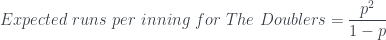
The expected number of runs per one-out inning for The Doublers

What if there was a team that only ever got doubles or strikeouts? No stolen bases or other base advances apart from on another hit, and no outs made on the bases. Let’s call this hypothetical team “The Doublers”.

For The Doublers, they don’t score until the second hit of the inning, and then they score one more run for every additional hit after that. If they get any runners on base, then they always leave one runner on base at the end of the inning. Their probability for scoring one run is the same as The Homers’ probability for scoring two runs; for two runs, the same as The Homers’ for three; etc. The expected runs per inning for The Doublers is therefore

$Expected\ runs\ per\ inning\ (Erpi)\ =\ 0(1-p) + 0p(1-p) + 1{p^2}(1-p) + 2{p^3}(1-p) + ... + (n-1){p^n}(1-p) + ...$

Let’s divide both sides by p:

$\dfrac{Erpi}{p} = 1p(1-p) + 2{p^2}(1-p) + ... + (n-1){p^(n-1)}(1-p) + ...$

The expression on the right hand side is the same one that we worked out before to equal p/(1-p). So now we have

$\dfrac{Erpi}{p} = \dfrac{p}{1-p}$

$Expected\ runs\ per\ inning\ for\ The\ Doublers = \dfrac{p^2}{1-p}$

Making sense of the difference between these two results

Now let’s think about this result for a moment. It’s exactly the expected runs for The Homers, but times p. This actually makes sense when you think about how The Doublers must reach a threshold of base reaches before they start scoring. Their first base reach nets them no runs, but after that, every base reach has the same result for The Doublers (one run scored) as does a base reach for The Homers. After reaching that threshold of one base reach, The Doublers’ expected runs for that inning become exactly the same as The Homers’ expected runs per inning for an inning that hasn’t started yet. It’s like that first baserunner is the “cost of admission” for The Doublers to begin scoring, and their chance of achieving that cost of admission is p, so we multiply The Homers’ expected runs of $\tfrac{p}{1-p}$ by the cost of admission $p$ to get The Doublers’ expected runs per inning of $\tfrac{p^2}{1-p}$ .

The expected number of runs per one-out inning for the other two teams

Now there are two more hypothetical teams we must consider: The Singlers and The Walkers. They’re just like The Doublers except The Singlers only hit singles, and more importantly they only hit them in such a way that it always takes exactly three base reaches to score the first run, and any additional runs also take three base reaches to get around. And The Walkers only get walks. In any inning in which they’ve reached their threshold, The Singlers will leave two runners on base, and The Walkers will leave three.

What are their expected runs per inning? We can sum up the probabilities for each possible number of runs as we did for The Homers and The Doublers, but we’ll get the same result as if we just multiply the probability of reaching their respective thresholds by The Homers’ expected runs per inning. For The Singlers, it takes two base reaches to reach their threshold, and because we only have one out per inning (in this hypothetical game, for now) those two base reaches must come from the first two batters. Since the chance of each batter reaching is $p$ , the chance of both reaching is $p^2$ . Multiply this by The Homers’ expected runs per inning and we get

$Expected\ runs\ per\ inning\ for\ The\ Singlers = \dfrac{p^3}{1-p}$

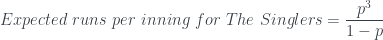
And by similar reasoning,

$Expected\ runs\ per\ inning\ for\ The\ Walkers = \dfrac{p^4}{1-p}$

Going from one-out innings to three-out innings

Well, that’s nice and tidy, but these are the expected run formulas for one-out innings. Baseball as it is played has three-out innings. So how will that change things? What do these formulas become when we switch to three-out innings?

There are actually a couple of ways we can go about this. We’ll start with the one that uses binomial theory, which is the way I originally did this. Then we’ll do it the way that provides more intuitive insight.

The probability of BR base reaches occurring in a 3-out inning

For all four hypothetical teams, we know the number of runs scored in the inning if we know the number of base reaches. For The Homers, runs scored r equals base reaches BR. For The Doublers, r=BR-1, except that r=0 if BR=0. For The Singlers, r is the greater of BR-2 or 0; for The Walkers, the greater of BR-3 or 0.

What is the probability of each of these numbers of base reaches? In our hypothetical in which all outs occur at the plate, there will be a mixture of BR base reaches and 2 outs, followed by one final out. Before that final out, there are a total of BR+2 plate appearances.

Binomial theory tells us the probabilities of what will happen when you repeat an event that has two possible outcomes. If one of those outcomes has a probability p, the other has a probability of 1-p. If you repeat the event N times, the probability of the outcome with probability p occurring exactly m times is

$\binom{N}{k}{p^k}{(1-p)^{N-k}}$

where $\binom{N}{k}$ is the binomial coefficient and equals $\tfrac{N!}{k!(N-k)!}$

(n! is “n factorial” and equals the product $n(n-1)(n-2)...$ )

In our case, the event that is repeated is a plate appearance; the two possible outcomes are a base reach and an out. So we use our count of plate appearances (PA=BR+2) for N, our count of base reaches (BR) for k, and our count of outs (2) for N-k. The probability of all these events occuring in any order in the inning, not including the final out of the inning, is therefore

$\binom{BR+2}{BR}{p^{BR}}{(1-p)^2}$

To get the overall probability of an inning having BR base reaches we must multiply this number by the probability of the occurance of the final out of the inning, which, as the probability that the last batter makes an out, is 1-p. The result is

$\binom{BR+2}{BR}{p^{BR}}{(1-p)^3}$

Now you may be wondering, why didn’t we take N as BR+3 instead of BR+2, as there are BR+3 plate appearances in the inning? It’s a very good question. The thing is that the binomial probability formula always accounts for both possible outcomes of each event. In this case, because the events are plate appearances, it accounts for both a base reach and for an out in each plate appearance we include. Say you’re talking about an inning with one base reach. In our all-outs-are-made-at-the-plate world, that means there will be four plate appearances in the inning. When will the base reach happen? In the first plate appearance? Possibly. Possibly not. In the second, or the third? Possibly, possibly not. In the fourth? That’s not possible, because the inning ends with the fourth batter, and innings always end with an out. So we can only use the binomial formula over those first three plate appearances. It considers all eight different ways that three plate appearances can go – including the possibilities of no base reaches, and the possibility of all three reaching base – and counts up how many of those eight have a total of one player reaching base. It produces the number three for that – that’s the first part of the formula, the

$\binom{3}{1}$

that gives us the three. Each of those three ways that things can go has a probability of $p^1(1-p)^2$ , so the formula is just adding up all the different probabilities for each way we can end up with one base reach over the first three batters. Then we must multipy this by the probability of (1-p) for the fourth batter having made an out, and we have the probability that the inning ends with only one base reach.

But what if that fourth batter doesn’t make an out? Sometimes he’ll reach base. That’s true. We don’t know that ahead of time. But we’re just counting up possibilites here, and the possibility of the fourth batter reaching base is counted up, just not as part of innings with only one base reach. It’s counted up in the probabilities of all innings with more than one base reach. In the end, if you add up all the probabilities we come up with for each number of possible base reaches in an inning, we should get the number 1. That’s if we did things correctly. Verifying this is a convenient way to check that we didn’t make some mistake along the way, so we’ll give it a shot here.

By using a shortcut. We need to take the sum:

$\sum_{BR=0}^{\infty} \binom{BR+2}{BR}{p^{BR}}{(1-p)^3}$

This is (1-p) times a diagonal of the binomial theory version of Pascal’s Triangle. There’s a relation that tells us that such diagonals added up give you the value 1/(1-p):

$\sum_{j=0}^{\infty} \binom{j+k}{j}{p^{j}}{(1-p)^k} = \dfrac{1}{1-p}$

If we use BR for j, and 2 for k, our sum of the probabilities of each inning with BR base reaches in it becomes

$\dfrac{1}{1-p}(1-p) = 1$

And that’s a pretty strong confirmation that we didn’t undercount or overcount any possible outcomes.

Expected number of runs per 3-out inning

Now we have the probability of BR base reaches in an inning. To get expected numbers of runs, we multiply each of these by the number of runs that will score for that number of base reaches, then add up all the products we get. We’ll do The Homers, The Doublers, The Singlers, and The Walkers all at once by assigning the letter L to the number of batters left on base for each (assuming they even make their threshhold). So L=0 for The Homers, 1 for The Doublers, 2 for The Singlers, and 3 for The Walkers.

In our fictional universe, everyone who reaches base either scores or is left on base at the end of the inning, so the number of runs scored in an inning with BR base reaches is BR-L. When multiply this by the probability for BR base reaches and sum, we get

$\sum_{BR=L+1}^{\infty} (BR-L)\binom{BR+2}{BR}{p^{BR}}{(1-p)^3}$

Note that we don’t start BR at 0 because any values of BR less than L would give a negative number of runs, which is incorrect. We don’t start at L either, because this gives 0 runs, which makes that term zero, and therefore contributes nothing to the sum. So we’re clear to start summing at BR=L+1 and going higher from there.

To make this expression useful, we need to convert this infinite sum into a finite expression of some sort. When I first worked on this formula, I used the only trick I knew for doing that, which was much more limited than the one I have now, and made for a very long, tricky derivation. I also derived each L value separately. Fortunately, we’ll have much better tricks we’ll be using here, and it will save us much greif.

The main trick we need is the following relationship for binomial coefficients:

$\sum_{j=c}^{\infty} \binom{j+k}{j}{p^{j}}{(1-p)^k} = \sum_{i=0}^{k} \binom{c-1+i}{c-1}{p^{c-1}}{(1-p)^i}, for c > 0$

(or for c=0, this equals $\dfrac{1}{1-p}$ , as we saw before).

If you look, our sum comes close to fitting the left hand side of this equation. Our summation index BR always takes a value of at least 1, so we will use the main part of this formula. With j = BR, c=L+1, and k=2, we match both the summation index, and the binomial probability $\binom{j+k}{j}{p^{j}}{(1-p)^k}$ (we must first factor out the (1-p) factor that we previously multiplied in, to get this to match). If we can pull the (BR-L) factor and the (1-p) factor outside of the summation, then we can apply the formula. We can factor out (1-p) because it does not depend on our index, BR; unfortunately, (BR-L) does depend on the index. But we have another trick for handling that; we can combine a portion of (BR-L) with the binomial probability, to produce a different binomial probability term that we can then apply our formula to.

First, we break up BR-L as follows:
BR-L = BR + 3 – 3 – L = (BR+3) – (L+3)

This will allow us to separate the summation into two summations, one with a (BR+3) factor and the other with a (L-3) factor. The (L-3) can be factored out of its summation, allowing us to use our formula on that one.
The remaining summation will contain $(BR+3) \binom{BR+2}{BR}{p^{BR}}{(1-p)^2}(1-p)$ . This we transform as follows:

$(BR+3)\binom{BR+2}{BR}{p^{BR}}{(1-p)^2}(1-p)$

$= (BR+3)\dfrac{(BR+2)!}{BR!2!}{p^{BR}}{(1-p)^2}(1-p)$

$= \dfrac{(BR+3)!}{BR!2!}{p^{BR}}{(1-p)^3}$

$= 3\dfrac{(BR+3)!}{BR!3!}{p^{BR}}{(1-p)^3}$

$= 3\binom{BR+3}{BR}{p^{BR}}{(1-p)^3}$

This is just 3 times a different binomial probability. So by factoring the 3 out of the summation, we will be able to use our formula on it.

Putting it all together:

$Expected\ runs\ per\ inning$
$= \sum_{BR=L+1}^{\infty} (BR-L)\binom{BR+2}{BR}{p^{BR}}{(1-p)^2}(1-p)$

$= \sum_{BR=L+1}^{\infty} [(BR+3) - (L+3)]\binom{BR+2}{BR}{p^{BR}}{(1-p)^2}(1-p)$

$= \sum_{BR=L+1}^{\infty} (BR+3)\binom{BR+2}{BR}{p^{BR}}{(1-p)^2}(1-p) - \sum_{BR=L+1}^{\infty} (L+3)\binom{BR+2}{BR}{p^{BR}}{(1-p)^2}(1-p)$

$= 3 \sum_{BR=L+1}^{\infty} \binom{BR+3}{BR}{p^{BR}}{(1-p)^3} - (L+3)(1-p)\sum_{BR=L+1}^{\infty}\binom{BR+2}{BR}{p^{BR}}{(1-p)^2}$

$= 3 \dfrac{p}{1-p} \sum_{i=0}^{3} \binom{L+i}{L}{p^L}{(1-p)^i} - (L+3)(1-p)\dfrac{p}{1-p} \sum_{j=0}^{2} \binom{L+j}{L}{p^L}{(1-p)^j}$

It may seem wise at this point to combine the terms of like index, because their binomial probabilities are identical, so will combine easily. That would leave the i=3 term in the first summation standing alone, uncombined. However, it turns out that it is better to combine terms that have the same exponent on their (1-p) factor. For that, we combine summation terms for which i-1 = j (so i=1 to j=0, etc.), and we let the i=0 term stand alone. This gives us

$Expected\ runs\ per\ inning$
$= 3 \dfrac{p}{1-p} \sum_{i=0}^{3} \binom{L+i}{L}{p^L}{(1-p)^i} - (L+3)(1-p)\dfrac{p}{1-p} \sum_{j=0}^{2} \binom{L+j}{L}{p^L}{(1-p)^j}$

$= 3 \dfrac{p}{1-p} \binom{L}{L}{p^L}{(1-p)^0} + \dfrac{p}{1-p} \sum_{i=1}^{3} [3\binom{L+i}{L}{p^L}{(1-p)^i} - (L+3)(1-p)\binom{L+i-1}{L}{p^L}{(1-p)^{i-1}}]$

$= 3 \dfrac{p}{1-p}{p^L} + \dfrac{p}{1-p} \sum_{i=1}^{3} [(3 \dfrac{(L+i)!}{L!i!}{p^L}{(1-p)^i}) - (L+3) \dfrac{(L+i-1)!}{L!(i-1)!}{p^L}{(1-p)^i}]$

$= \dfrac{p}{1-p}{p^L} (3 + \sum_{i=1}^{3} [(3 \dfrac{L+i}{i} - (L+3)) \dfrac{(L+i-1)!}{L!(i-1)!}{(1-p)^i}] )$

We can simplify that first portion of the summation as follows:
$(3 \dfrac{L+i}{i} - (L+3))$

$= \dfrac{3(L+i) - (L+3)i}{i}$

$= \dfrac{3L + 3i - Li - 3i}{i}$

$= \dfrac{L(3-i)}{i}$

$Expected\ runs\ per\ inning\ =\ \dfrac{p^{L+1}}{1-p} (3 + \sum_{i=1}^{3} [\dfrac{L(3-i)}{i} \binom{L+i-1}{L}{p^L}{(1-p)^i}] )$

The (3-i) factor makes the i=3 term zero, so we can drop it from the summation:
$Expected\ runs\ per\ inning\ = \dfrac{p^{L+1}}{1-p} (3 + \sum_{i=1}^{2} [\dfrac{L(3-i)}{i} \binom{L+i-1}{L} (1-p)^i] )$

The “3” is exactly what you get in the summation expression for i=0, so we can absorb it into the summation. And that first L within the summation can be absorbed into the binomial coefficient, modifying it.
$Expected\ runs\ per\ inning\ = \dfrac{p^{L+1}}{1-p} \sum_{i=0}^{2} [(3-i)\binom{L+i-1}{L-1}(1-p)^i]$

Writing out the summation leads to our final result:
$Expected\ runs\ per\ inning\ = \dfrac{p^{L+1}}{1-p} (3 + 2L(1-p) + \dfrac{1}{2}L(L+1)(1-p)^2)$

Going from three-out innings to innings of any number of outs

We could have just started plugging in values for i a few steps back, but I wanted to also show the formula you can get when you don’t assume 3 outs per inning, but instead a variable number of outs per inning. If the number of outs per inning is OPI, then the formula you get just changes in two places:

$Expected\ runs\ per\ inning\ = \dfrac{p^{L+1}}{1-p} \sum_{i=0}^{OPI-1} [(OPI-i)\binom{L+i-1}{L-1}(1-p)^i]$

If you check by plugging in OPI=1 and OPI=3, you’ll see that this gives us the formulas we’ve already derived for both 1-out innings and 3-out innings. And so now with this formula we can answer questions such as “How would run production be affected by changing the number of outs in an inning to 4?”.

Writing out the different component formulas

Let’s write those out here. The EBP component formulas for 1-out innings are
$EBP(p,L) = \dfrac{p^{L+1}}{1-p}$

For 3-out innings are
$EBP(p,L) = \dfrac{p^{L+1}}{1-p} (3 + 2L(1-p) + \dfrac{1}{2}L(L+1)(1-p)^2)$

For 4-out innings areEBP(p,L)
$EBP(p,L) = \dfrac{p^{L+1}}{1-p} (4 + 3L(1-p) + L(L+1)(1-p)^2 + \dfrac{1}{6}L(L+1)(L+2)(1-p)^3)$

Let’s expand these out for each possible value of left on base, allowing L to take the values 0, 1, 2, and 3.

For 1-out innings:

$Expected\ runs\ per\ inning\ for\ The\ Homers\ (L=0)\ = \dfrac{p}{1-p}$
$Expected\ runs\ per\ inning\ for\ The\ Doublers\ (L=1)\ = \dfrac{p^2}{1-p}$
$Expected\ runs\ per\ inning\ for\ The\ Singlers\ (L=2)\ = \dfrac{p^3}{1-p}$
$Expected\ runs\ per\ inning\ for\ The\ Walkers\ (L=3)\ = \dfrac{p^4}{1-p}$

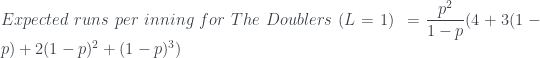
For 3-out innings:
$Expected\ runs\ per\ inning\ for\ The\ Homers\ (L=0)\ = \dfrac{p}{1-p}\ 3$
$Expected\ runs\ per\ inning\ for\ The\ Doublers\ (L=1)\ = \dfrac{p^2}{1-p} (3 + 2(1-p) + (1-p)^2)$
$Expected\ runs\ per\ inning\ for\ The\ Singlers\ (L=2)\ = \dfrac{p^3}{1-p} (3 + 4(1-p) + 3(1-p)^2)$
$Expected\ runs\ per\ inning\ for\ The\ Walkers\ (L=3)\ = \dfrac{p^4}{1-p} (3 + 6(1-p) + 6(1-p)^2)$

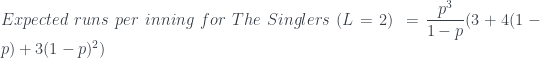
For 4-out innings:
$Expected\ runs\ per\ inning\ for\ The\ Homers\ (L=0)\ = \dfrac{p}{1-p}\ 4$
$Expected\ runs\ per\ inning\ for\ The\ Doublers\ (L=1)\ = \dfrac{p^2}{1-p} (4 + 3(1-p) + 2(1-p)^2 + (1-p)^3)$
$Expected\ runs\ per\ inning\ for\ The\ Singlers\ (L=2)\ = \dfrac{p^3}{1-p} (4 + 6(1-p) + 6(1-p)^2 + 4(1-p)^3)$
$Expected\ runs\ per\ inning\ for\ The\ Walkers\ (L=3)\ = \dfrac{p^4}{1-p} (4 + 9(1-p) + 12(1-p)^2 + 20(1-p)^3)$

The 3-out-inning formulas and 4-out-inning formulas are the same as the 1-out-inning formulas, multiplied by an additional factor. This is why I call this additional factor the “outs-per-inning multiplier”. This is explained more fully in The meaning of each part of the EBP formulas.

Producing runs-per-plate-appearance and runs-per-base-reach versions

Two other ways of measuring run production that I have found more useful and interesting than runs per inning are runs per plate appearance and runs per base reach. With our idealized assumptions, it’s a simple matter to convert our runs per inning formula into a runs per plate appearances formula. First, convert to runs per out by dividing by three (or by the number of outs per inning – OPI – for your rules). Then, multiply by outs per PA to convert the denominator to PA. Because Outs per PA is just 1-p, we therefore multipy by 1-p. So multiplying by that, we get

$Expected\ runs\ per\ plate\ appearance = \dfrac{p^{L+1}}{3} [3 + 2L(1-p) + \frac{1}{2}L(L+1)(1-p)^2]$

To get the runs per base reach formaula, we can divide runs per PA by base reaches per PA. Base reaches per PA is just p, so dividing the runs per PA formula by p gives
$Expected\ runs\ per\ base\ reach\ =\ \dfrac{p^L}{3} [3 + 2L(1-p) + \frac{1}{2}L(L+1)(1-p)^2]$

Or more generally, for a game of baseball played with OPI outs per inning:

$Expected\ runs\ per\ plate\ appearance = \dfrac{p^{L+1}}{OPI} \sum_{i=0}^{OPI-1} [(OPI-i)\binom{L+i-1}{L-1}(1-p)^i]$
$Expected\ runs\ per\ base\ reach\ =\ \dfrac{p^L}{OPI} \sum_{i=0}^{OPI-1} [(OPI-i)\binom{L+i-1}{L-1}(1-p)^i]$

This gives us three different versions of the EBP component formula. Because at times we’ll want to distinguish between the three versions, or be clear which one we’re referring to, we’ll create a unique identifier for each. We’ll use
$EBP_{IN}$ for the runs per inning formula,
$EBP_{PA}$ for the runs per plate appearance formula, and
$EBP_{BR}$ for the runs per base reach formula.

Next step: deriving how to linearly combine the four formulas

As explained in the introductory article to EBP, to model real teams we must take our four component formulas and add together fractions of each of these. For the fractions, we use the percentage of the time that we expect the team to leave L=0, 1, 2, or 3 runners on base in an inning. We use formulas that predict what each of these fractions is expected to be. Each fraction gets its own unique formula – some extremely simple, others very complex.

For a demonstration of the derivation of these formulas, see Full derivation of Expected Binomial Production left-on-base fractions.

The Baseballsphere Blog

The (sometimes mathematical) baseball thoughts, analysis, and ideas of Tom McIntyre

Full derivation of Expected Binomial Production component formulas

Beginning with the simplest case

The chance of The Homers scoring n runs in a one-out inning

The expected number of runs per one-out inning for The Homers

The expected number of runs per one-out inning for The Doublers

Making sense of the difference between these two results

The expected number of runs per one-out inning for the other two teams

Going from one-out innings to three-out innings

The probability of BR base reaches occurring in a 3-out inning

Expected number of runs per 3-out inning

Going from three-out innings to innings of any number of outs

Writing out the different component formulas

Producing runs-per-plate-appearance and runs-per-base-reach versions

Next step: deriving how to linearly combine the four formulas

Beginning with the simplest case

The chance of The Homers scoring n runs in a one-out inning

The expected number of runs per one-out inning for The Homers

The expected number of runs per one-out inning for The Doublers

Making sense of the difference between these two results

The expected number of runs per one-out inning for the other two teams

Going from one-out innings to three-out innings

The probability of BR base reaches occurring in a 3-out inning

Expected number of runs per 3-out inning

Going from three-out innings to innings of any number of outs

Writing out the different component formulas

Producing runs-per-plate-appearance and runs-per-base-reach versions

Next step: deriving how to linearly combine the four formulas

Share this:

Like this: